Mind the risk: The value of valuations

Forecasting asset returns is a tricky business. For example, in a recent blog, I outlined some of the pitfalls when interpreting scatter plots of realised returns against valuation metrics.

But even if we are confident in our expected return estimates, it can be easy to forget that this is only half the story.

A common motivation for forecasting time-varying expected returns is to tilt portfolios through time, as opposed to maintaining a static allocation. However, in responding to changes in market conditions, it’s not just changes in expected return investors might wish to pay attention to. Investors may also wish to pay attention to changes in risk.

An example

This is possibly best illustrated by a simple example. Suppose for illustration that there are just two assets to invest in – a riskless asset and a risky asset – and two states of the market, A and B. States A and B have the following statistics for the risky asset:

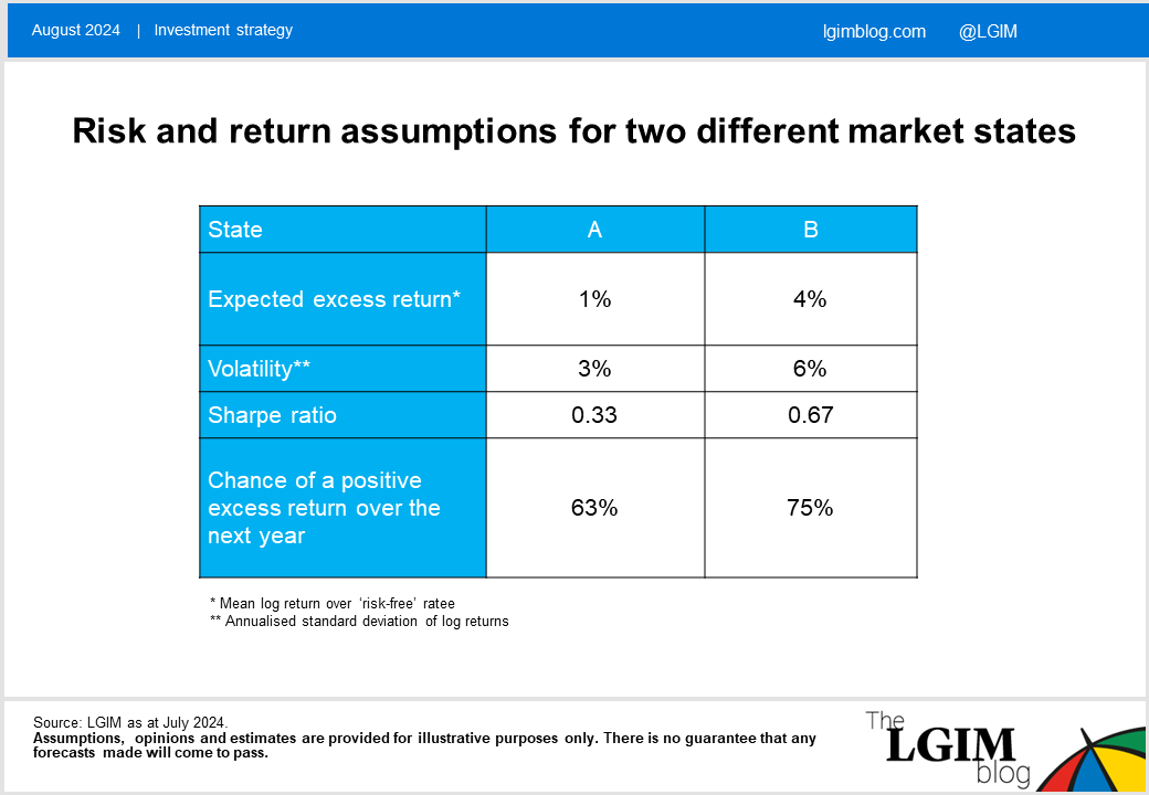
We assume a two-year investing horizon with returns in the second year uncorrelated to those in the first. In the first year you know you’re in state A, whereas in in the second year you know it’s flipped to state B.

The question is: given your insight into the market, how can you most efficiently allocate over your investing horizon?

You’d be forgiven for being strongly tempted to adopt a higher allocation to the return-seeking asset in year 2, when the market is in state B. Relative to state A, it has four times the expected excess return and double the Sharpe ratio. It would therefore seem easy to argue that it’s become a more attractive proposition than it was in the first year.

But this is misleading. The most efficient strategy could actually be a static percentage allocation over both years, with any tilting damaging efficiency.

Wait … really?

You may be sceptical of this claim, so I ran some simulations[1] to illustrate the point:

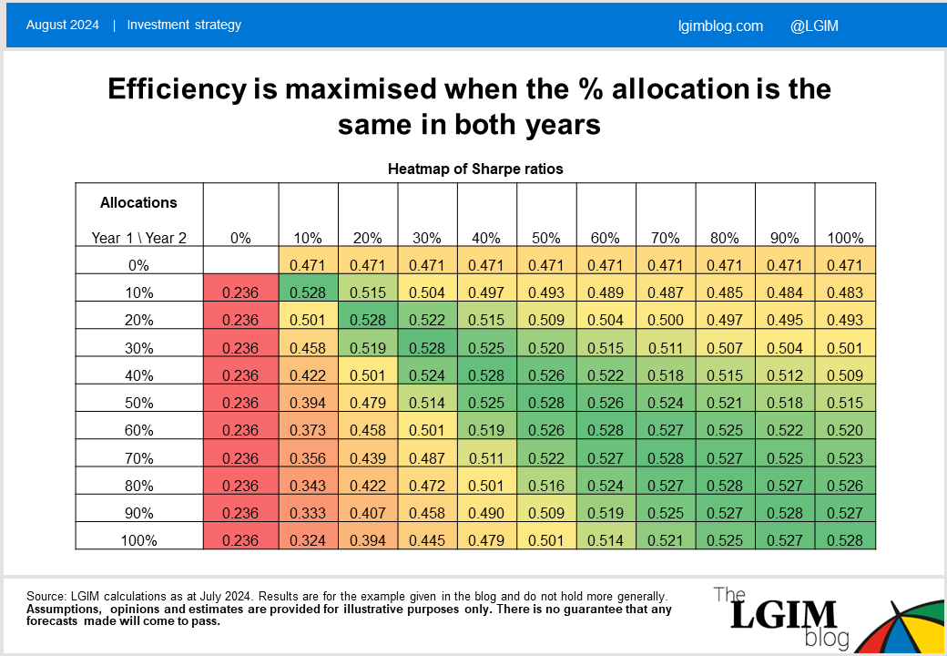
The leftmost column is the percentage allocation to the risky asset in year 1, when the market is in state A. The top row is the percentage allocation to the risky asset in year 2, when the market is in state B. Each number in the heatmap then represents the Sharpe ratio over the two-year period.

As you can see efficiency is maximised along the diagonal i.e. when you have the same percentage allocation in year 2 as year 1. According to this model, if you want a higher or lower expected return, the most efficient way to do this is to increase or decrease your percentage allocation to the risky asset in both years.

The maths underpinning this is that the ideal strategy involves setting the percentage allocation in proportion to the expected excess return, but inversely proportional to the square of the volatility^[2]. Expected excess return here has quadrupled on moving from state A to state B, but the doubling of volatility cancels this out (given 2 squared is 4).

What could this help explain?

In a blog a couple of months ago, we looked at some backtests and simulations of credit exposure, and found it was difficult to boost efficiency by holding more credit when spreads were wider (and less when they were tighter), despite a clear and strong relationship between spread levels and average future excess returns. The situation above is far simpler than the messy reality there[3], but can help explain some of the challenge.

With the benefit of hindsight, market crashes can appear to fantastic opportunities. However, we shouldn’t forget that the heightened expected returns at these points are almost invariably accompanied by increased risk, and it doesn’t take much of an increase in risk to nullify any perceived benefits of tilting towards the asset in question.

Similarly, low future expected returns are unappealing in themselves, but it doesn’t take much of a decrease in risk to justify remaining invested.

None of the above is to say that the market is not prone to bouts of optimism or pessimism that are unwarranted based on fundamentals. But it does remind us to pay attention to risk as well as return, and may give us pause for thought before assuming a change in strategy is necessarily the right response to a change in valuations.

 

Past performance is not a guide to the future. The value of an investment and any income taken from it is not guaranteed and can go down as well as up, you may not get back the amount you originally invested. Assumptions, opinions and estimates are provided for illustrative purposes only. There is no guarantee that any forecasts made will come to pass.

[1] I calculated using 1,000 scenarios. However, I was also able to replicate the results using formulae.

[2] Under quadratic utility, investors should size their risk exposure in proportion to the Sharpe ratio.

[3] For example, returns in adjacent years are negatively correlated.